Note:This blog assumes that you have a basic understanding of Pytorch and convolutions in general.Now onto LeNet-5.

The Story of LeNet-5

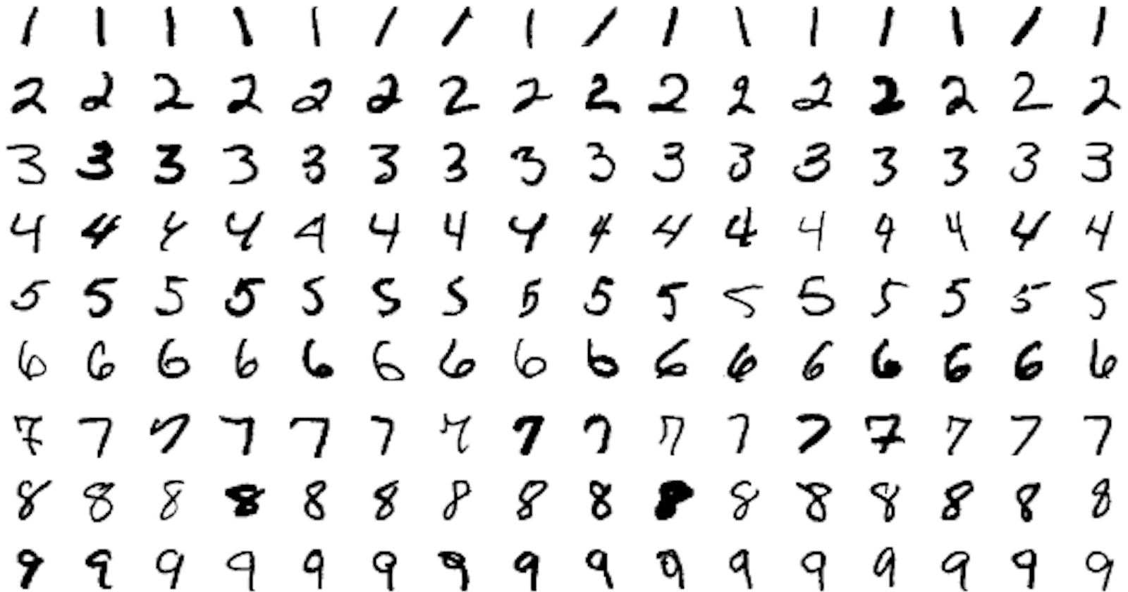
I was trying to understand about how convolutions work and came across LeNet - 5. It was developed in 1998 by Yann LeCun et al., LeNet-5 was a groundbreaking achievement in its time. It successfully tackled the challenging task of handwritten digit recognition on the MNIST dataset, achieving an impressive accuracy of around 99%. This feat paved the way for the widespread adoption of CNNs in various image-related applications.There are many new variations in convolutions used currently but we can consider LeNet-5 as the foundational convolutional model even though it was not the first one which was developed in 1989.

Architecture Explanation:

Convolutional Layer 1(C1): takes an input of 32 x 32 pixel image with using 6 feature maps or filters of size 5 x 5 with stride 1 and converts it into a 28 x 28 pixel image.

Pooling(S2): The subsampling layer or the pooling layer has a size of 2 x 2 with stride 2 which converts the input(28 x 28) into a 14 x 14 pixel image.

Convolutional Layer 2(C3) : takes an input of 14 x 14 pixel image with using 16 feature maps or filters of size 5 x 5 with stride 1 and converts it into a 10 x 10 pixel image.

Pooling(S4): The subsampling layer or the pooling layer has a size of 2 x 2 with stride 2 which converts the input(10 x 10) into a 5 x 5 pixel image

Convolutional Layer 3(C5): takes an input of 5 x 5 pixel image using 120 feature maps or filters of size 5 x 5 with stride 1 and converts it into a 1 x 1 pixel image.

Feedforward Layer(F6): is a simple neural network layer with 84 hidden units (120,84)

Output Layer: outputs the 10 scores or the predictions of the input.

Pytorch Implementation:

Step 1: Imports.

'''In this case for torchvision.transforms i am not using torchvision.transforms.v2 which is the latest version in pytorch'''
import torch,torchvision
from torch.utils.data import DataLoader
from torch.utils.data import sampler
import torch.nn as nn
import torch.nn.functional as F
import torchvision.transforms as T
import torchvision.datasets as Datasets

Step 2: Device Initialisation.

if torch.cuda.is_available():
  device = torch.device('cuda')
else:
  device = torch.device('cpu')
print(f'Using device = {device}')

Step 3 : Data preprocessing.

We will split the data here for train(training data),val(validation data) and test(testing data) where train will be used during training and val for accuracy.The test dataset will be used for the final accuracy and predictions of the model.

Note:The MNIST in Pytorch's vision datasets has the split only for train and test.So the we have to split the train data which is 60000 into 59000 for train and 1000 for validation. We will make no changes in the test data(10000) which Pytorch provides.

transforms_train = T.Compose([T.ToTensor(),
                        T.Resize((32,32)),
                        T.Normalize(mean = (0.1307,),std = (0.3081,))])
transforms_test = T.Compose([T.ToTensor(),
                        T.Resize((32,32)),
                        T.Normalize(mean = (0.1325,),std = (0.3104,))])
batch_size = 64
NUM_TRAIN = 59000
train = Datasets.MNIST(root = 'data',
                       train = True,
                       transform = transforms_train,
                       download = True)
train_data = DataLoader(train,batch_size,sampler=sampler.SubsetRandomSampler(range(NUM_TRAIN)))
val = Datasets.MNIST(root = 'data',
                      train = True,
                      transform = transforms_train,
                      download = True,
                          )
val_data = DataLoader(val,batch_size,sampler=sampler.SubsetRandomSampler(range(NUM_TRAIN,60000)))
test = Datasets.MNIST(root = 'data',
                     train = False,
                     transform = transforms_test,
                     download = True)
test_data = DataLoader(test,batch_size,shuffle = True)

Lets Understand the above code better by breaking each part:

Data Transformations:

transforms_train = transforms.Compose([
    transforms.ToTensor(),  # Convert to tensors (CHW format)
    transforms.Resize((32, 32)),  # Resize to 32x32, as required by LeNet-5
    transforms.Normalize(mean=(0.1307,), std=(0.3081,))  # Normalize based on mean and standard deviation
])

transforms_test = transforms.Compose([
    transforms.ToTensor(),
    transforms.Resize((32, 32)),
    transforms.Normalize(mean=(0.1325,), std=(0.3104,))
])

• transforms.ToTensor(): Converts the images to PyTorch tensors, where each channel (red, green, blue) is represented as a 3D tensor in our case this value is 1 as it is a grayscale image.

• transforms.Resize((32, 32)): Resizes all images to a uniform size of 32x32 pixels. This is done because LeNet-5 was specifically designed to work with 32x32 input images. Resizing ensures that all images contribute equally to the training process .

• transforms.Normalize(mean=(0.1307,), std=(0.3081,)): Normalizes pixel values using the calculated mean and standard deviation of the MNIST dataset. Normalization helps to improve the stability and convergence of the training process, as it scales pixel values to a smaller range, often between 0 and 1. This can make the learning process more efficient.(The code for finding the mean and std will be in the colab file on my github)

Creating DataLoaders:

batch_size = 64
NUM_TRAIN = 59000
train = Datasets.MNIST(root = 'data',
                       train = True,
                       transform = transforms_train,
                       download = True)
train_data = DataLoader(train,batch_size,sampler=sampler.SubsetRandomSampler(range(NUM_TRAIN)))
val = Datasets.MNIST(root = 'data',
                      train = True,
                      transform = transforms_train,
                      download = True,
                          )
val_data = DataLoader(val,batch_size,sampler=sampler.SubsetRandomSampler(range(NUM_TRAIN,60000)))
test = Datasets.MNIST(root = 'data',
                     train = False,
                     transform = transforms_test,
                     download = True)
test_data = DataLoader(test,batch_size,shuffle = True)

• datasets.MNIST(): Loads the MNIST dataset from the specified root directory (usually 'data'). The train argument controls whether to load the training or testing set. The transform argument applies the defined transformations to each image.

• batch_size=64: Specifies the number of images to process in each batch during training and validation.

• SubsetRandomSampler: Creates samplers that select a subset of indices from the original dataset. This is used to split the training set into a smaller training set and a validation set.

• shuffle=True: Shuffles the test data to ensure that the model is evaluated on a randomly ordered set of images.

Step 4 : Analyse the data.

for x,y in train_data:
  print(x.shape,y.shape)
  break

Output for the following code is :

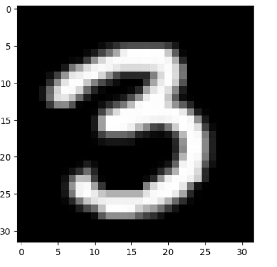
Now the shape of x is 64,1,32,32 where 64 is the batch size , 1 is the number of channels in case of grayscale images the channels or depth is only 1 but in case of coloured images the depth is 3 and 32 x 32 are the pixels of our image.

import matplotlib.pyplot as plt
plt.imshow(x[0].squeeze(),cmap = 'gray')
plt.show()

Step 5 : Creating the model

class LeNet(nn.Module):
   def __init__(self,):
      super().__init__()
      self.C1 = nn.Conv2d(1,6,5,1)
      nn.init.kaiming_normal_(self.C1.weight)
      self.S2 = nn.MaxPool2d(2,2)
      self.C3 = nn.Conv2d(6,16,5,1)
      nn.init.kaiming_normal_(self.C3.weight)
      self.C5 = nn.Conv2d(16,120,5,1)
      nn.init.kaiming_normal_(self.C5.weight)
      self.fcl1 = nn.Linear(120,84)
      nn.init.kaiming_normal_(self.fcl1.weight)
      self.fcl2 = nn.Linear(84,10)
      nn.init.kaiming_normal_(self.fcl2.weight)
   def forward(self,x):
      x = F.relu(self.C1(x))
      x = self.S2(x)
      x = F.relu(self.C3(x))
      x = self.S2(x)
      x = F.relu(self.C5(x))
      x = torch.flatten(x,1)
      x = F.relu(self.fcl1(x))
      x = self.fcl2(x)
      return x

Lets understand the code linearly:

Initialization:

1. Class Definition:

   • LeNet(nn.Module): Inherits from nn.Module for PyTorch's neural network functionalities.

2. Module Attributes:

   • C1: First convolutional layer (1 input channel, 6 output channels, 5x5 kernel, stride 1).

   • S2: max pooling layer (2x2 kernel, stride 2).

   • C3: Second convolutional layer (6 input channels, 16 output channels, 5x5 kernel, stride 1).

   • C5: Third convolutional layer (16 input channels, 120 output channels, 5x5 kernel, stride 1).

   • fcl1: First fully connected layer (120 input units, 84 hidden units).

   • fcl2: Second fully connected layer (84 input units, 10 output units).

3. Weight Initialization:

   • nn.init.kaiming_normal_(weight): Applies the Kaiming Normal initialization to all convolutional and fully connected layer weights. This is a common initialization technique that aims to improve training convergence.

Forward Pass:

1. Convolution and ReLU:

   • x = F.relu(self.C1(x)): Passes the input through the first convolutional layer followed by ReLU activation.

2. Max Pooling:

   • x = self.S2(x): Applies max pooling with a 2x2 kernel and stride 2 to downsample the feature maps.

3. Repeat Steps 1-2:

   • The same operations (convolution, ReLU, max pooling) are repeated for C3 and S2 again.

4. Third Convolution and ReLU:

   • x = F.relu(self.C5(x)): Applies a third convolutional layer with 120 filters, followed by ReLU activation.

5. Flatten:

   • x = torch.flatten(x, 1): Flattens the 3D feature maps into a 1D vector before entering the fully connected layers.

6. Fully Connected Layers:

   • x = F.relu(self.fcl1(x)): Passes the flattened features through the first fully connected layer with 84 hidden units and ReLU activation.

   • x = self.fcl2(x): Passes the output of the previous layer through the second fully connected layer with 10 output units (for the 10 digits).

Output:

• The final x represents the model's predictions, a 10-dimensional vector.

• Note : We can use softmax to present the 10 dimensional vector as probabilites but in this case we are just outputing scores.

Step 6 : Creating the training and accuracy loop.

def train_model(loader,model,optimizer,epochs = 1):
  model = model.to(device)
  for e in range(epochs):
    for t,(x,y) in enumerate(loader):
      model.train()
      x = x.to(device)
      y = y.to(device)
      logits = model(x)
      loss = F.cross_entropy(logits,y)
      optimizer.zero_grad()
      loss.backward()
      optimizer.step()
      if t % accuracy_interval == 0:
        print(f'Epoch = {e + 1}')
        print(f'Iteration {t} , loss {loss.item():.4f}')
        test_model(val_data,model)
        print()

def test_model(loader,model):
  if loader.dataset.train:
        print('Checking accuracy on val set')
  else:
        print('Checking accuracy on test set') 
  num_correct = 0
  num_samples = 0
  model.eval()
  with torch.no_grad():
    for x,y in loader:
      x = x.to(device)
      y = y.to(device)
      logits = model(x)
      pred = logits.argmax(1)
      num_correct += (pred == y).sum()
      num_samples += len(pred)
    acc = float(num_correct)/num_samples
    print(f'Got {num_correct}/{num_samples} correct {100*acc:.4f} ')

Lets Understand both the functions separately:

1.train_model(loader, model, optimizer, epochs=1):

• Purpose: Trains the model for a specified number of epochs (epochs) using the provided data loader (loader), model (model), and optimizer (optimizer).

• Steps:

  1. Move model to device: Ensures the model resides on the device (e.g., GPU) for efficient computation.

  2. Epoch loop: Iterates for the specified number of epochs (e).

  3. Batch loop: Iterates over each batch (t) in the data loader .

  4. Move data to device: Transfers input data (x) and target labels (y) to the device.

  5. Forward pass: Generates predictions (logits) from the model.

  6. Calculate loss: Computes the cross-entropy loss between predictions and labels.

  7. Optimize: Clears gradients (optimizer.zero_grad()), backpropagates loss (loss.backward()), and updates model parameters (optimizer.step()).

  8. Print training progress: Occasionally (every accuracy_interval iterations), prints epoch, iteration, and current loss.

  9. Evaluate on validation set: Periodically runs test_model on the validation data for performance monitoring (not shown in provided code).

2.test_model(loader, model):

• Purpose: Evaluates the model's performance on a given data loader (loader).

• Steps:

  1. Identify dataset: Prints whether evaluating on the validation or test set based on the loader's dataset train attribute.

  2. Set model to evaluation mode: Deactivates dropout and batch normalization for proper prediction.

  3. Disable gradient calculation: Use torch.no_grad() context to prevent unnecessary memory usage during evaluation.

  4. Loop over data: Iterates through each batch (x, y) in the loader:

  5. Calculate and print accuracy: Computes final accuracy (acc) and prints the number of correct predictions, total samples, and accuracy percentage.

Step 7 : Running the model:

model = LeNet()
optimizer = torch.optim.SGD(model.parameters(),lr = 1e-3)
train_model(train_data,model,optimizer,epochs = 10)

We instantiate the model with using the optimizer as Stochastic Gradient Descent and then we train the model for 10 epochs.

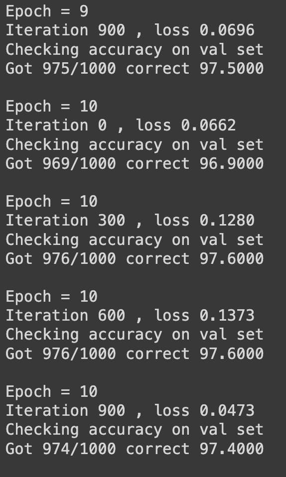
In the end we got an accuracy for 97.4% for 10 epochs.We can try to increase our accuracy by using various other methods such as batch normalization ,dropout,etc.

Wrapping Up:

In this blog, we've delved into the iconic LeNet-5 architecture. We've implemented it from scratch in PyTorch, covering the essential steps of model definition, data preparation, training, and testing.

This blog is meant to be an intro for someone who wants to implement LeNet 5 architecture and it is also a start to document my learnings in public.

I hope it was helpful :)

References:

1.Yann LeCun's lecture.

2.Andrej Karpathy's Lecture.

3.GradientBased Learning Applied to Document Recognition.